
Trending

Written by: Marc Odo | Swan Global Investments
Comparing Hedging and Options Strategies
One recent innovation that has taken the financial marketplace by storm is buffered outcome ETFs. Also known as defined outcome, target outcome, or structured outcome, these strategies have found an audience with investors who wish to have some upside potential with their investments but are wary of a market sell-off. According to Morningstar, there are well over 100 ETFs with over $8bn in AUM as of August 2021. All of this has occurred within the last three years.
Buffered Outcome ETFs
Most buffered outcome ETFs employ some version of a trade known as a put-spread collar. Therefore, referring to our post on put-spread collars will help in understanding buffered ETFs.
A buffered outcome ETF typically has four components:
- A long, deep-in-the-money call position to give the ETF market exposure
- A long put to hedge the downside
- A short, out-of-the-money call
- A short put that is further out of the money than the long put
The premium collected from the two short positions (i.e. #3 and #4) is used to offset the cost of the hedge (#2). Often these trades are constructed to be “zero cost”, meaning the premium collection from the two short positions is meant to net out the cost of the hedge as closely as possible.
This begets the question: “If most buffered outcome ETFs use this basic put-spread collar trade, how can there be so many different products on the market?”
It is true that buffered outcome ETFs share many core characteristics. Across the range of 100+ products, there are more similarities than differences. That said, the primary difference in the various buffered ETF products has to do with the trade-off between upside and downside. How much upside does a buffered ETF have before it is capped out versus how much downside does the ETF experience before the hedge start to prevent losses? There are dozens of variations of buffered outcome ETFs designed for outcomes ranging from conservative to aggressive.
The language that has been developed to detail the differences regarding buffered outcome ETFs usually focuses on the protection range. It is usually communicated as two numbers such as 5/20 where the first number indicates the amount that the investor will lose in a market decline up to that number (i.e., deductible). The second number indicates the end of the protection zone where the investor will match further market losses.
So, in plain English, if someone described a buffered product as “5/20”, then within the defined outcome period, that investor:
- could expect to lose 5% in their investment if the market was down 5%;
- would be sheltered from losses in the market beyond 5%, up until;
- the market is down 20%. If the market continues to drop beyond 20% the investor is exposed to those losses.
There are many variations on this theme. We used 5/20 as an example, but 0/15, 5/35, 0/9 are all possible pay-offs too. There is really no limit to the way these buffered outcome ETFs can be structured, which is why there are so many on the market.
The astute reader might ask, “If the points where the protection begins and ends are defined, then what about the cap? Why isn’t that specified?”
The answer is the cap is usually the variable in the equation. These trades are often established with the goal of being “zero cost”, meaning that the cost to purchase the long put is offset by the premium gained by writing the short put and the short call. If the strike prices of two of these three positions are set in stone, that means the third position, the short call, must be a variable. The strike price is a “plug” number to keep the two sides of the equation in balance. In plain English, sometimes the cap will be set higher, sometimes the cap will be lower. It just depends on market conditions.
Drivers of Returns
The primary driver of returns for buffered outcome ETFs will simply be the returns of the underlying asset, in most cases the S&P 500. What matters, however, is the direction and the scale and of the returns.
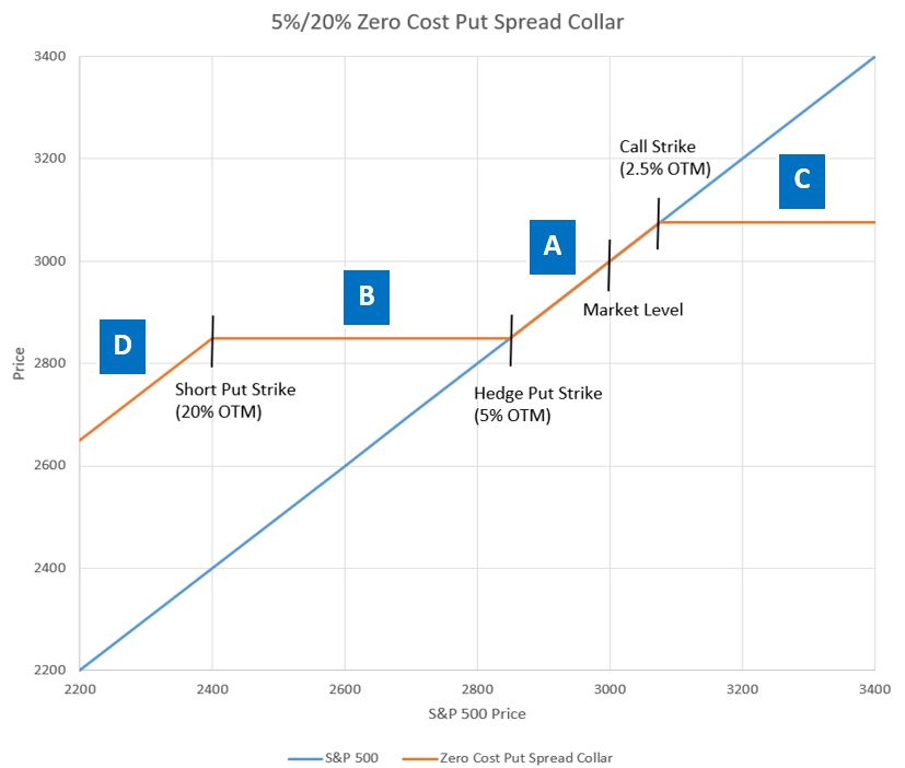
Assuming that the buffered ETF is utilizing a simple put-spread collar trade, the following could be expected:
- If the returns on the market are up or down by a modest amount [zone “A”], then the buffered ETF is expected to have a return in line with the underlying asset over the specified time frame (usually one year);
- If the market breaks through the upside cap [ zone “C”], then the buffered ETF flat-lines and receives no further upside returns.
- To the downside, once the market falls past the first inflection point the buffered ETF should be sheltered from further losses [zone “B”], up until the point of the second inflection point.
- After the second inflection point [zone “D”] the buffered ETF’s return will be fully exposed to further losses in the market. Please see our post on put-spread collars for further explanation.
Risks in a Buffered Outcome ETF
The risks to most buffered ETFs lie in the extremes.
- If the market is up a lot, the buffered ETF will not enjoy gains beyond a certain point [zone “C” in the chart above].
- If markets sell off too much, the buffered ETF is exposed to open-ended losses [zone “A” in the chart above).
The former is an opportunity cost and the latter is a very real risk to capital.
In addition, it should be noted that the specific returns advertised by these products are almost never realized given that those returns rely on investment on a specific date and holding the investment through expiration (e.g., one year). Investors who join after the launch or leave the series before the end of the period may receive far different returns. The structured returns are only there for investors who invest on a particular date and then stay the entire time.
Role of Buffered Outcome ETFs in a Portfolio
As mentioned previously, a vast number of variations of buffered products have been released over the last few years. This is both a good thing and a bad thing. On a positive note, there are variants of the buffered ETFs to fit just about any risk profile, from very conservative to very aggressive. If an investor has a specific buffer in mind, odds are that someone has an ETF to match.
On the downside, this means the investor must really do their due diligence and understand the trade-offs between upside potential and downside risks before investing in a particular strategy. Also, as all the “basic” variations of buffered outcome strategies have been released, many ETF companies are developing the next generation of buffered ETFs that might be more exotic than a basic put-spread collar. These variations might have risks that differ significantly from a basic put-spread collar and might impact an investor portfolio in unexpected ways.
How Do Buffered ETFs Compare to the DRS?
Swan Global Investments manages many different types of hedged equity and options-based strategies. In addition, Swan has partnered with Pacer ETFs to provide investors with a family of buffered outcome ETFs. Swan has been managing its proprietary hedged equity strategy called the Defined Risk Strategy since its inception in 1997.
The Defined Risk Strategy shares a few similarities with buffered outcome ETFs, as they are both hedged equity solutions that offer some market upside combined with downside risk mitigation.
However, the primary difference is the Defined Risk Strategy is actively managed whereas buffered outcome ETFs are passively managed. Buffered products are “set it and forget it,” where once a year the put-spread collar trade is established. There is no recourse for the manager to adjust positions in these strategies to minimize losses or take advantage of market conditions without violating the implicit contract represented by the structured/buffered outcome value proposition. If the market blows through either the call strike price (to the upside) or the put strike price (to the downside) a buffered ETF will not take any action.
Alternatively, Swan’s Defined Risk Strategy (DRS) actively manages the re-hedging of the portfolio.
- If the markets decline significantly, Swan will look to monetize the hedge and acquire additional equity shares at reduced prices (i.e., sell high, buy low). The re-hedge process differentiates Swan’s DRS from other strategies and is critical to long-term full market cycle performance in the DRS.
- If markets are up significantly within a calendar year, the DRS does not have a hard-stop to gains, like buffered ETFs do. Swan will look to move the hedge upwards to lock-in a portion of the market gains, but unlike buffered outcome ETFs the gains are not sold away via a short call position.
- Finally, if the market doesn’t make a significant move up or down within the span of a year, the DRS will look to sell its long put option hedges while there is still some value associated with them. A buffered ETF that does not see its put option go in-the-money with a market decline will have that option expire worthless at the end of one year.
In summary, Swan’s Defined Risk Strategy is actively managed and is designed for full market cycles using a disciplined process to address some of the weaknesses of traditional hedged equity option strategies and capitalize on large market declines.
Related: Implications for Equity Investing at Historic Valuations